Predicting risk of money laundering activity using semi-supervised methods
In the gambling industry, money laundering is one of the most threatening concerns for any operator. It is a rare event but can introduce severe fine from the gambling authorities if a case goes unchecked/unreported. In the recent past, machine learning has become increasingly successful in identifying such events in online gambling. In this article, we focus on explaining the implementation of semi-supervised methods to generate risk predictions.
Here, we first describe the modelling objectives with a little summary of anomaly detection. The next section covers limitations, assumptions and modelling approach in this process. And finally, the results section illustrates the outcome of the algorithms evaluated over a dummy dataset.
Objectives
In the financial risk domain, it is improbable to build an exceptional solution that identifies all known patterns. Also, the problem scope is extensive to be embraced by one model. Hence, we have the following composite solution to approach the money laundering problem.
-
Identify any change in the account from its historical behaviour. (for simplicity, we named it Local anomaly detection). This implementation is available in our previous post.
-
Identify accounts that are anomalous when compared to a population. (Global anomaly detection)
Anomaly Detection is a method to identify an outlier in a dataset. Traditionally, the following two types are acknowledged.
-
Novelty detection (Semi-supervised)
The training data is not polluted by outliers and, we are interested in detecting whether a new observation is an outlier. In this context, an outlier is also called a novelty.
-
Outlier detection (Unsupervised)
The training data contains outliers which are defined as observations that are far from the others. Outlier detection estimators thus try to fit the regions where the training data is the most concentrated, ignoring the deviant observations.
More details on the novelty and outlier detection are available on scikit-learn documentation.
Our objective is to identify money laundering activity, and we also have access to labelled data points. Therefore, it is reasonable to train a model for novelty detection in the data. Accordingly, we explored the following methods for what we referred to as global anomaly detection.
- Ensemble-based algorithms
- Isolation forest and Robust random cut forest
- Density-based algorithm
- LOF (Local outlier factor)
- Neural Networks
- Autoencoders
There are tons of articles available online on the implementation of these algorithms. Here, we intend to describe an approach that successfully analyses these models within the Gambling industry.
Limitations
-
Unavailability of external data.
Every licensed online casino/gaming platform has a mandatory department of analysts to review accounts for money laundering activities. It is a manual process that also includes a lot of external data such as credit checks etc. This dataset is not available for all customers and hence is not usable for modelling purposes.
-
Bias in positive labels.
A positive label is assigned after the successful manual evaluation of an account. Therefore, each datapoint suffers from the selection/knowledge bias due to the complex understanding of the assessment rules.
Another business constraint is the market-specific regulations on deposits and gambling activities. Each gambling authority has its own rules and regulation for risk analysis. For example, the deposit limit can vary between Sweden and the UK. Therefore, a business with the dominant customer base in one market biases the estimates of any model.
In this work, we have not taken any action to mitigate this bias.
Assumptions
-
Customers typically have a fixed budget.
It is reasonable to assume that people turning towards gaming/betting as entertainment come with a fixed budget. It is one of the decisive checks in the evaluation process and is also called affordability check.
-
Customers have limited gaming behaviour.
Given the infinite number of options to choose for betting and gaming, typically, customers stick to selected few sports and games. It is due to the constraints of personal interest and knowledge requirement to be successful in different sports. This assumption enables us to compare distinct gaming behaviour within a population.
Modelling Procedure
-
Feature selection
Like any other machine learning model, feature selection is the key in this analysis. We have divided the features into three parts.
-
Financial transactions such as deposits, withdrawals, and banking methods. (more info on this is available here under section features)
-
Gaming behaviour: stakes, number of bets, bet frequency and safe bets.
-
Verification data: Verified emails, other documents and country of residence.
One can better understand the importance of these and other required features by following the FATF guidelines and Gaming authorities regulations. One such document for the Swedish market is available here
We have split each relevant feature into six time-based windows such as deposit/withdrawal amount, gaming behaviour etc. It helped us capture the change over time and introduced an implicit time-bound characteristic in the model. The following table shows the segments used to create time-based features.
24-hour 48-hours 14-days 3-months 6-months lifetime The 24-hour segment corresponds to the last active date of an account. The 48-hour segment was computed before the last active day. Other segments follow the same routine i.e. calculated over the account duration before the last active date. This division enabled isolating the recent customer behaviour in the model and is crucial for evaluating newly registered accounts with limited history. It also removes bias in the features with an odd recent activity such as very high deposit amount.
-
-
Data Preprocessing
The model data includes more than 200 features generated via the time-segmentation process using financial, gaming and verification data segments. It composed of the following three parts where development and test set also contains a
labelcolumn.-
Train dataset
-
Development dataset and,
-
Test dataset
The training dataset does not contain any known positive data point for novelty detection models. However, the dev and test sample includes positive labels via the bootstrap sampling strategy. The contamination value determines the number of positive data points in a given sample.
Contamination is the proportion of outliers in the data set.
This strategy helped us create better dev and test set for model evaluation. The contamination value is also required for the RRCF algorithm as it defines the number of examples in a tree. This value can also be tuned as a hyper-parameter. However, we have estimated this value from the population and kept it constant at 0.001.
-
-
Hyperparameter tuning
We implemented the grid search method to find the best possible parameters for each model. The same fraction of the training dataset is used in model training for all algorithms. Also, the number of evaluation sample remains the same throughout the process.
-
Evaluation metric
The primary metric is the average AUC value measured over precision and recall through cross-validation on the dev set. To better understand the distribution of these values, we have included the standard deviation of AUC.
AUC (Area Under the ROC Curve) provides an aggregate measure of performance across all possible classification thresholds. One way of interpreting AUC is the probability that the model ranks a random positive example more highly than a random negative example.
More explanation on AUC/ROC metric is available at Google machine learning crash-course
Algorithms
Now we have developed a framework to implement and evaluate different models. In this section, we briefly introduce the following four algorithms with links for further reading. Our intent with this post is to provide a structure to compare these algorithms within the Gambling industry.
-
Ensemble-based
The Isolation Forest and RRCF follow the notion that the anomalies are expected to be different only over a few dimensions than the normal data points.
-
Isolation Forest
The IsolationForest ‘isolates’ observations by randomly selecting a feature and then, randomly selecting a split value between the maximum and minimum values of the selected feature. Since recursive partitioning can be represented by a tree structure, the number of splittings required to isolate a sample is equivalent to the path length from the root node to the terminating node.
Implementation details of this algorithm can be found on scikit-learn and relevant papers are available using the following links, Isolation Forest and Isolation Based Anomaly Detection.
-
Robust Random Cut Forest (RRCF)
RRCF was introduced as an improvement over isolation forest to detect anomalies in streaming data. However, this is quite useful in batch applications as well.
As defined in the Amazon SageMaker
The RCF algorithm organizes the data in a tree by first computing a bounding box of the data, selecting a random dimension (giving more weight to dimensions with higher variance), and then randomly determining the position of a hyperplane cut through that dimension.
The only open-source python implementation is available at python projects. While the original paper is available here
This StackOverflow answer provides a decent explanation of the differences between RRCF and iForest.
-
-
Density-based
-
LOF (Local Outlier Factor)
It measures the local deviation of the density of a given sample with respect to its neighbours. It is local in that the anomaly score depends on how isolated the object is concerning the surrounding neighbourhood.
Implementation details for scikit-learn can be found here.
-
-
Neural-Networks
-
Autoencoders
These are the type of artificial neural network that is applied to learn the representation of data. The objective of an autoencoder is to encode-decode the dataset to remove noise and reduce dimension. The model first compresses the data to decrease dimensions through a bottleneck layer. Then in the decompression stage, data is recreated using the compressed lower-dimension space.
Since the anomalies do not follow a similar pattern as the normal data points, they get the highest noise/reconstruction error. Therefore, the high error value is the representation of an irregularity in the data. Here are few links to follow more details on autoencoders, intro to autoencoders, stanford tutorial and, keras blog.
-
Results
A synthetic dataset is used for hyperparameter/tuning process using CV to compute average AUC over precision and recall values. This dataset follows a similar distribution as observed in the real-world application. The following steps describe the model evaluation process.
- Train all models on the same fraction of training data.
- Generate
ndev samples (as defined in the data pre-processing step). - Compute average AUC and std AUC values.
The complete implementation of this process and sample data used in this analysis are available on GitHub. The code employs the python multiprocessing module to improve performance on a single machine. The Tensorflow implementation of autoencoders uses Ray for improving hyperparameter tuning. We have also provided a wrapper for distributed model training of the RRCF algorithm. Using the current open-source implementation, it trains an RRCF forest on a single processor.
Using the framework explained above, we have observed the following results.
| Algorithm | Average AUC value | SD AUC value |
|---|---|---|
| Isolation Forest | 0.0930 | 0.022 |
| LOF | 0.0038 | 0.00013 |
| RRCF | 0.7060 | 0.035 |
| Autoencoder | 0.3800 | 0.050 |
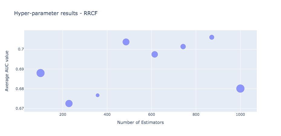
The RRCF performed best across all investigated solutions. However, due to current open-source implementation, the model training is slow and highly resource depleting. Nevertheless, this solution has demonstrated potential in the high dimensional problem domain. The graph below shows the average AUC value for the different estimators. The scatter point size on the plot is controlled by the sd AUC value.
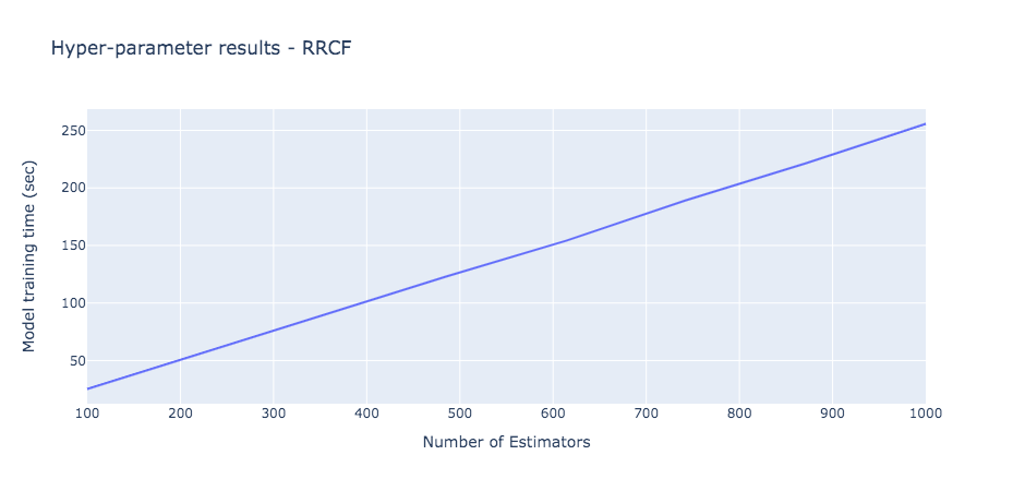
The model training time of RRCF for a sample 1000 data point is displayed below.
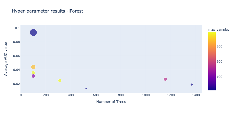
The Isolation Forest model provided the best average AUC value of ~0.1 on the given sample. We believe with better hyper-parameters and more data points, the performance of this model will be better.
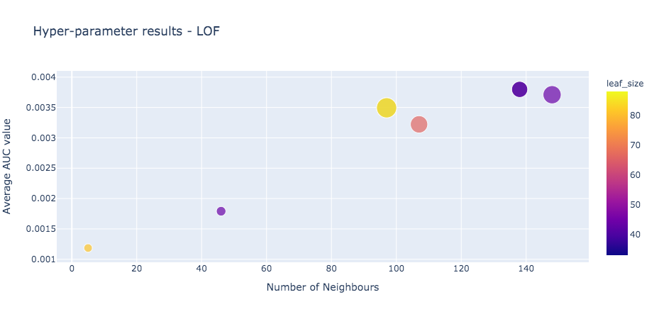
The density-based LOF model showed the weakest performance in our analysis.
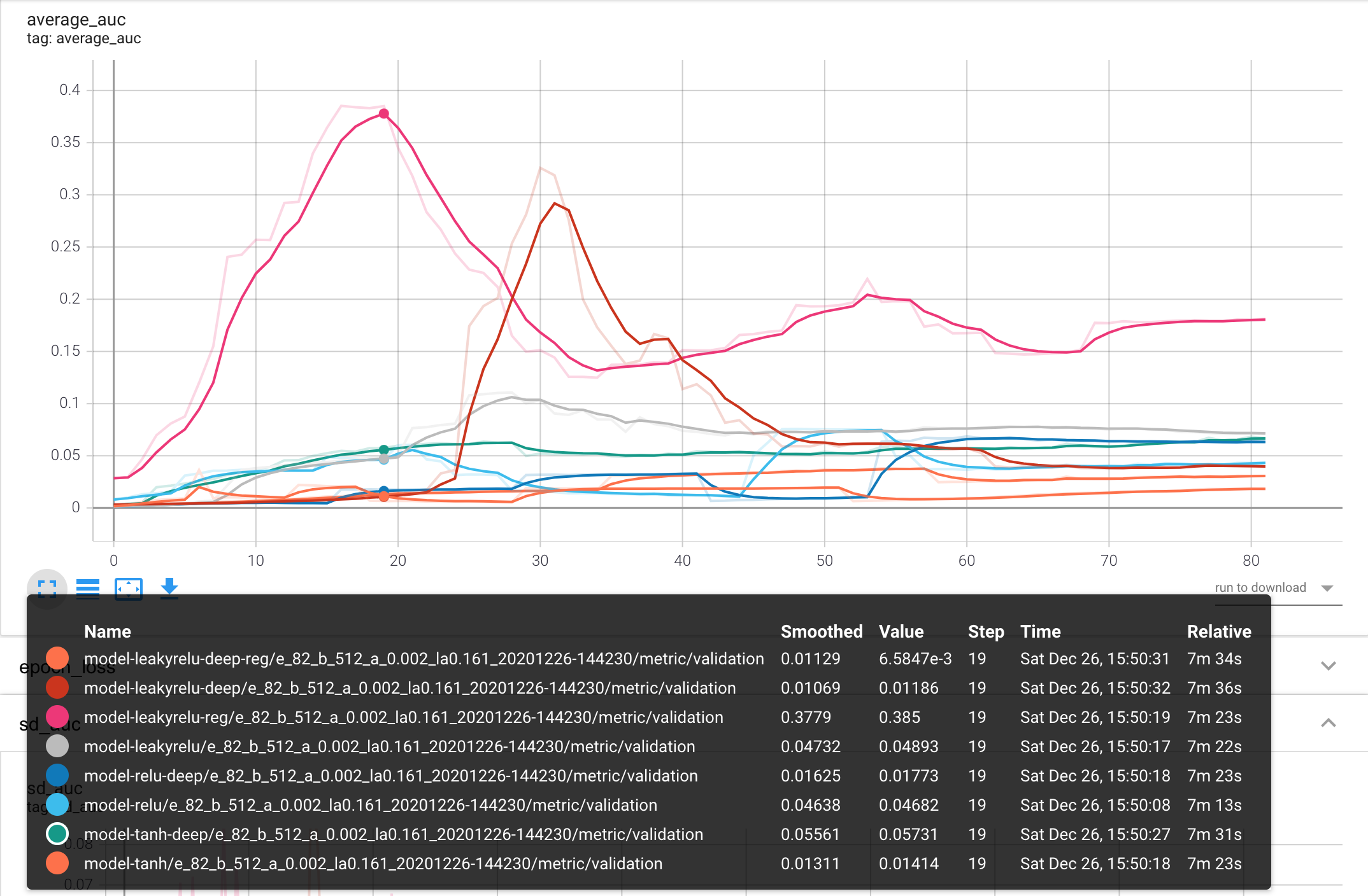
We have evaluated eight different network architecture to solve the rare event detection problem. The shallow autoencoder model with only three layers of an encoder, bottleneck, and a decoder performed the best. This model used leaky-relu activation function with l2 regularization.
Conclusion
We evaluated four Novelty detection algorithms using a dummy dataset within the Gambling industry. Below is a summary of the outcome of this analysis.
- The ensemble-based model, RRCF performed best on the given dataset. Although, the current open-source python implementation is not scalable on larger datasets.
- The density-based model, LOF failed to perform satisfactorily. It also has a slow and inefficient performance over large datasets.
- Autoencoders showed potential when evaluated over a small sample. Though, these models have very long training and model tuning process that also require bigger datasets.
- Therefore, due to current scalability/performance issues, we have discounted the LOF and RRCF results. Hence, we will favour Autoencoders as the model of choice for this analysis. (To analyse the scalability, we have replicated the current dataset to generate a more extensive input. However, the implementation is not addressed in this post. Readers are free to investigate this using the given dataset or any other dataset of their own.)
Future work
In future, we would like to explore better configurations of Autoencoders and other Neural Network models such as LSTM.
Another aspect is to mitigate the market influenced bias in the model where the trained model is likely to perform better in a specific market.